Understanding MagVIT2: Language Model Beats Diffusion:
Tokenizer is key to visual generation

Hi! Welcome to my almost weekly blog post. And thanks to huggingface reading group for keeping me motivated to keep doing this. Today we are looking at the paper “Language Model Beats Diffusion: Tokenizer is key to visual generation”. The code for this is here by the legend lucidrian and they seem to have some training results training on music. This is a pretty important paper that caused Open Source communities like LAION to be very excited as this is a competitive approach to diffusion which is way easier to connect to large language models with image generation. In fact, in this paper, they also explore video generation. Now let us investigate how they do this.
VAEs

Now, firstly let us explain what AE(Autoencoders) are. These models take images, let’s say they are 512 by 512, and compress them to 64 by 64 encoding/latent space or even smaller while ensuring we can reconstruct them decently. These models are trained to make the reconstruction, obtained from the latent space, as close to the original as possible.
Now, VAEs go a bit beyond that where we ensure that even if we change the encoded 64 by 64 by adding a small bit of noise we can still reconstruct similar images. See that there is no such guarantee for the autoencoder! You can encode a cat, but if you add a bit of noise you can decode a car. VAEs were made so that the latent space/encoded space has some useful meaning to us that we can understand. In other words, Variational Autoencoders are robust to “variation”. For more info, I recommend checking out this blog!
VQGANs

VQGANs and VQVAEs were ideas made to bring VAEs to the next level. In particular, people thought why don’t we make VAEs output words? However, you might be wondering, how is this possible? Images are continuous values to an extent. They are not like texts which are discrete values. And this is very true.
What VQVAEs did was very simple. VQ stands for Vector Quantize. What this means is that we make an embedding of say 4096 words. Then we encode the image into a vector, let’s say v. Then, we find the closest embedding in our 4096 words to that v and replace v with that! Now, if our decoder can output the original image well enough, then we now have an encoder that can tokenize all images into words! One note, we can see that this is a VAE because it is pretty robust to variations!
Language Modeling

Now, we have represented images as words so now, can we do something like ChatGPT where we can just generate a bunch of words/image tokens and output images? The answer is yes. If we were to check out a huggingface project, open-muse is a project that attempts to reproduce a Google model that does exactly that.
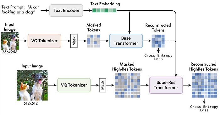
It’s a bit like the above but the main idea is during training, we encode the image as tokens, then we mask out a portion of those tokens, and then we train our model to predict those masked tokens! Then, from a completely masked output 64 times 64 tokens, we can gradually unmask those tokens to get a good final image!
Issue with VQVAEs/VQGANs
However, one common issue present was that all these language modeling approaches were just worse than say doing diffusion models like stable diffusion. This research paper found that the reason for this is that VQGAN’s representation is just not a good representation of the visual world. In that, even when reconstruction quality increases, generation quality doesn’t necessarily improve. For example, in the above case, you can see that if you are having trouble describing images with only access to 256 words, we can train a VQGAN model with access to 1024 words instead. This helps reconstruction but when we combine this with a language model, after a certain point, increasing the number of words/vocabulary hurts performance! Below is a graph of this

As an alternative, the authors propose a new model called Lookup-free quantizer(LFQ).
LFQ
Originally, in VQGAN, we had each word have embeddings the size of some embedding dimension that we matched our encoded image against. However, here, that dimension is reduced to 0. And as you can guess from the name, Lookup-free quantizer, the need for finding the closest embedding is gone too which is a huge computation save. The only part common with VQGANs is that the vocabulary has a fixed size. How this works is as follows:
First, let us imagine our vocabulary as an array of -1 and 1s like so -1, 1, 1, 1, -1.
Then, how many words do we have in the vocabulary? Since we have 2 choices at each index it will be 2*2*2*2*2=2⁵ in the above case.
Now, when we quantize say a latent of 5 dimensions, then we want to find if the index i of our latent is closer to -1 or 1, or choosing the index in an array of {-1, 1}. If it’s closer to -1 we say at index i, we choose 0 and if it’s closer to 1, we way at index i we choose 1. Now let z at index i be zᵢ
Then, we can just say if zᵢ ≤ 0 we choose 0 and otherwise we choose 1! Now, if we do this for all 5 dimensions we get something like
0, 1, 0, 0, 1
which looks very much like binary! And then, once we convert the above to natural numbers, in this case, 9, we can say 9 is our token.
With this change, as can be seen by the graph above, increasing the vocabulary consistently decreased language modeling loss which is pretty impressive.
Aside on Entropy
Now, if we just train an LFQ like the above, what typically happens is that the model learns to not prioritize all the tokens but just a subset of them for short-term gain and just forget about all else. This was an issue even during VQGANs. To combat this, we revisit a notion called entropy
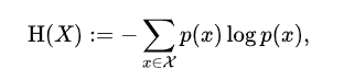
Where the basic idea is at every index we calculate the probability of that index times the log of that probability. Now, I won’t go much into the theory of this but we want to maximize this. When we do we will have all tokens appearing at roughly equal probability(test it out!), thus our model will learn to use all tokens!
However, the authors didn’t want the tokens to be completely randomly distributed. More so they wanted the tokens to have clustered in that there are some meaningful token groups that are together. To do this they made the loss

The first part is just as we explained before maximizing the spread across all tokens, but we deduct the entropy of the average binary representation. My understanding of the second term is we are reducing the randomness of how the average tokens look. So we are clustering while doing our best to spread individual images throughout those clusters. The authors mainly got this idea from this paper which was also a very interesting read!
Video Generation
I am very new to this part so let me know if any part doesn’t make sense! Now, the existing method that was used to do something like VQGAN on videos was C-ViViT
C-ViViT

The main idea seems that first, we encode the first frame of the video. Then, with a spatial transformer, we capture the spatial relations in the image. Now, this was just for the first frame but in future frames, all the previous frames are very important in describing it. So now, we have a causal transformer that looks over all the processed frames from the spatial transformer and outputs tokens!
While this performs well, when we use transformers, we use something called positional embedding to tell the model which position the current token is. So as long as the spatial transformer is right there, as it labels which part of the frame is at which position, it forces the model to only work with fixed-resolution videos. Additionally, the authors of Magvit2 found that using 3d cnns just performs better.
MagVIT2 Improvements
So, now the new design is to just remove the spatial transformer with a 3d CNN like so
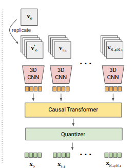
However, we are still left with a causal transformer. Will it be possible to replace even this and put all the encoding parts into one model? This was the exact same question the authors had and the answer is yes
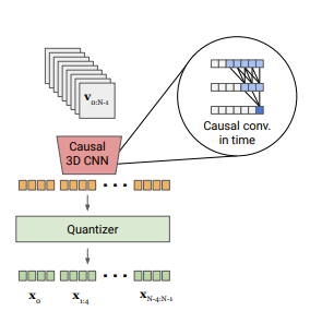
They made a new model called a Causal 3d CNN. My understanding of this Causal 3d CNN is instead of doing regular convolution over the frames with some kernel size k, the convolution kernel only “looks back” in time. In that we do not look at k/2 frames in the future and k/2 frames in the past, we look at k frames in the past which makes the outputs more “causal”. In the end, this tokenization performed best for the authors!
This blog turned out way more dense than I planned but hope you all enjoyed it! I think I’ll add results later if I get time but the overall conclusion seems like it’s just better than previous approaches