Understanding “Common Diffusion Noise Schedules and Sample Steps are Flawed” and Offset Noise


This blog post is inspired by the GitHub user https://github.com/bghira who is in Huggingface discord and Laion discord with the tag @pseudoterminalx. He made a model based on the research paper “Common Diffusion Noise Schedules and Sample Steps are Flawed” which you can play around with in this colab notebook. As you can see from the above images, and zooming in, the details are pretty incredible. While composition-wise some alternate techniques are similar, for small details like the hair and the small textures on the iguana, you will have a hard time achieving similar results with other models. The exact reason for this is that most of them have a fundamental flaw of not completely denoising images and are usually left with some “noise” in the final output.
For example, let us ask models to generate “a solid black background”. Then, given SDXL v1.0 on the top left, playground v2 on the top right, bghira’s model, Terminus, on the bottom left and Deepfloyd IF on the bottom right

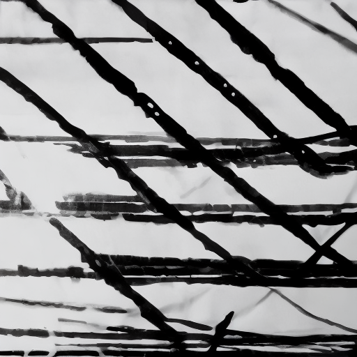
While Deepfloyd IF seems the closest, which we will explain why in this blog, the only model that can successfully make a completely black image is Terminus! And feel free to test for yourselves! On default stable diffusion, I was always left with some noise like below.

However, the authors of the paper “Common Diffusion Noise Schedules and Sample Steps are Flawed” from Bytedance were not the first ones to discover this problem. The first people to find this were the people at Crosslabs in this very interesting blog post here. The technique Crosslabs made to solve this issue was called “offset noise”.
Offset Noise
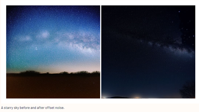
The authors of offset noise originally observed that it was very hard to make the output of stable diffusion models significantly dark or bright. The outputs tend to have an average of 0.5 which is right in the middle of completely white images and completely black images with a grayish texture.
The author of the blog originally tried to fine-tune a stable diffusion model on completely black images and even after many steps the output was like below
so the conclusion is that these stable diffusion models cannot generate completely black images. Now, why is this? The answer is that the objectives of training and inference are different in diffusion models. For this let us talk a bit about diffusion models.
Diffusion Models
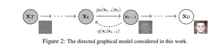
Diffusion Models have a forward process to add noise to the image and a reverse process to denoise the image. In diffusion models we also have timesteps. At timestep T we have complete noise and at timestep 0 we have the output image.
The forward/noising process is defined as so
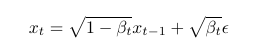
so we have the less noisy image, we multiply this by the square root of 1 minus some constant. And then we add a square root of that constant times ϵ!
Now, in typical stable diffusion models, the βₜ goes from 0.00085 for 0 timestep to 0.012 for T timestep. This means that at the beginning like x₀, x₁ we add very small amounts of noise but as we get closer to pure noise at the end, we ramp up the noise added.
Now, given the above formula, with a bit of math tricks, which you can check out here under how to train a diffusion model, we set αₜ = 1-βₜ, and we find
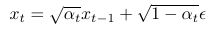
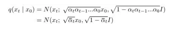
which means
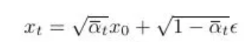
so we can go to a random timestep t from the original image at timestep 0 in just one go!
Diffusion Model Training Objective
Now, whenever we train a diffusion model, we choose a random timestep t and then noise up the image to get xₜ. Then from xₜ and timestep t, we predict ϵ that was used! The pseudo-code is below
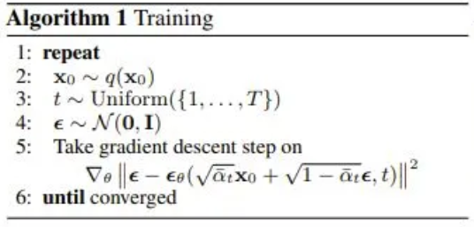
Diffusion Model Inference Objective
Now, for inference, the objective is we start with pure noise, and then for T timesteps we keep asking the model what the ϵ is and we go to the previous timestep until we reach 0! In pseudo-code this is
Discrepancy?
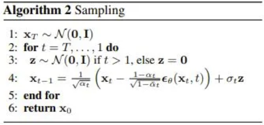
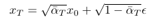
Now, did you catch the discrepancy? It is very subtle. We did mention before that βₜ goes from 0.00085 for 0 timestep to 0.012 for T timestep. Then, when we use
we can predict x at timestep T from x at timestep 0. Remember, we want this x at timestep T to be complete noise so ideally, it’s just ϵ. However, when the Bytedance Authors checked, this evaluated to
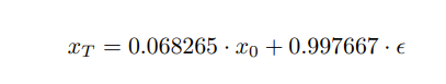
Now, that is very close to what we want but it’s slightly off. During training, even at timestep T, the model is expecting a tiny piece of the information from the original image to be present. On the other hand, for inference, we don’t provide an original image, we start with pure noise! So the model is looking for information in pure noise during inference which is not present.
The result of this discrepancy is very interesting. The Crosslabs blog author found that the information that remains of the original image which the model relies on to denoise, is the low-frequency information like the outlines of subjects while more tiny details, like textures, are destroyed.
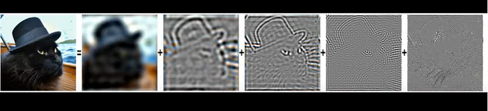
which does make sense. So the model looks for the low-frequency outlines in the latent noise and then relies on it for generation. One interesting feature of this that the Crosslabs author found was this is the reason for multiple images with different prompts but the same seed looks similar, they have the same low-frequency features.
Now, how can we fix this?
Back to offset noise
For the training objective, they set the initial noise added to be the below
noise = torch.randn_like(latents) + 0.1 * torch.randn(latents.shape[0], latents.shape[1], 1, 1)instead of the usual
noise = torch.randn_like(latents)Now, to understand this, it’s important to check the shapes!
torch.randn(latents.shape[0], latents.shape[1], 1, 1)has shape [batch size, channels, 1, 1]. So essentially, when we add this to
torch.randn_like(latents)we add a random normal distribution number to the latent width times the latent height number of pixels to have a different mean than 0! So essentially across all channels and batches, the normal distribution will have a different mean than 0 for all of them.
Now why will this help? Well, the main hint is that the lowest frequency information is the mean. To get intuition on this think of the waves below
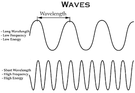
So, the highest frequency information will have a lot of occurrences across the image and is generally responsible for textures. For low-frequency information, they can occur very rarely. Now, there can be a low-frequency wave where the wavelength is larger than the image! In this case, we might be able to approximate the mean as part of this wave! This is called the zero-frequency component as it is a wave but it’s so long that basically, when it passes through the image, it’s basically just adding a constant.
Once this is done and Crosslabs retrained the model to take in offset noise, and then the model learned to ignore low frequency information more like below
so now dark images are possible.
However, one important fact to note is that this is fundamentally a hack. We are not resolving the issues with schedulers we are just side stepping them. The solution came in the paper we mentioned called “Common Diffusion Noise Schedules and Sample Steps are Flawed”
Common Diffusion Noise Schedules and Sample Steps are Flawed
The solution is very simple. Given below
why don’t we just move, alpha_bar_T,

to 0? And that’s exactly what they did
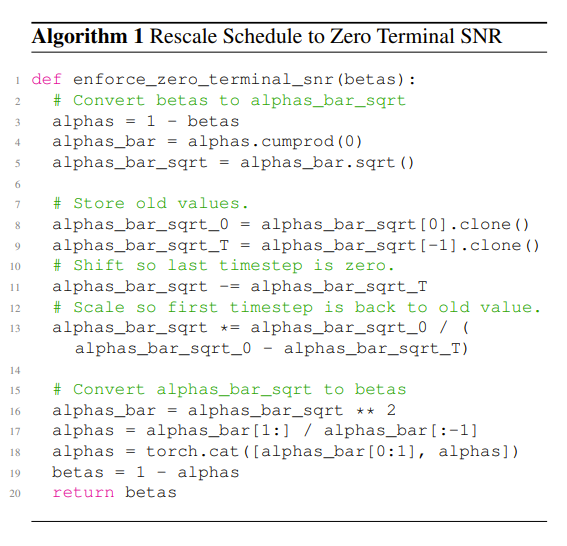
Basically, the above script sets the last timestep alpha bar to 0 and then reverse engineers the betas from it! Now observe here that we also made alpha at timestep T 0. However, now we have a new problem. Since we made it so that at timestep T, there is absolutely no information of x₀, during training, if we go to timestep T and have our model predict what noise was added, it’ll never have any idea. Regardless of what noise was added, we will always get total noise at timestep T. So, essentially at timestep T we will have an unsolvable learning problem!
To fix this, we need to look into V Prediction
V Prediction
V Prediction was first proposed in “Progressive Distillation for Fast Sampling of Diffusion Models” by Google.
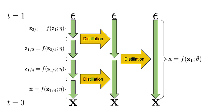
The idea was given a teacher model that can predict the next timestep we might be able to distill 2 of those teacher’s steps into one student step! And if we continue going then we will be able to directly predict our original image from pure noise!
For this problem, the authors also found difficulty with using epsilon prediction/predicting the noise added. The main reason is very similar to what we said above. The reasoning is
- During training, any ϵ that gets added will make x at timestep T pure noise since in this paper they assume alpha bar T is 0 at timestep T
- We want to do distillation on this so that we can predict the original image(x at timestep 0) from x at timestep T.
- From our epsilon prediction objective of predicting the noise added to the image at timestep 0, this is entirely useless in this one-step distillation because any noise can do that.
So the Google author proposed a series of strategies for a proper loss in this setting and one of the best-performing one was the v prediction.
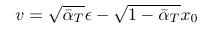
The formulation of v is

which with our notation is
Now, how this can be used to predict x like the above is written in Appendix D and it is pretty fascinating I recommend checking it out they did connect the above function with trigonometry!
Now, given this formulation, let us look at what happens when alpha bar t is 0. We are predicting the original image! Then, even in the case of our fixed scheduler, we now have a proper objective that doesn’t break at timestep T.
However, there can still be some slight discrepancy in inference compared to training even after all this is fixed.
Some slight flaws in sampling
Now, usually in training we train on 1000 steps but do inference on around 20 steps. Here, in most common implementations, in those 20 steps, the timestep T is not included! My understanding of this is to avoid 0 division errors but when we fix the scheduler, we need the first step to always be T. Now recall
since we trained our model on having alpha bar at timestep T be 0, alpha at timestep T is 0. Thus, our model learned to completely ignore the initial noise at timestep T and focus on making good ϵ to add. However, if we skip the initial timestep T, then we are adding the pure noise, which was supposed to be ignored, to our outputs! So essentially, during inference, we are adding noise to our generated output by not sampling from timestep T first!
Now, I heard that the above is still an issue with the diffusers implementation but I haven’t looked into it so let me know if anyone finds out!
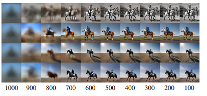
One interesting side effect of the above is that the output of the first timestep is always the same! Check out the output of timestep 1000 below!
Rescaling Classifier Free Guidance
For an explanation of classifier-free guidance, check out here
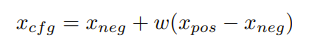
But the main idea is we try to push away from the default output of our model without text, x neg, towards the output of the model with text, x pos.
While that is all nice and good, the authors found that when they do this with their model, the output becomes overexposed interestingly. The authors claim this is because of the alpha bar T going to 0. My guess for why this is is as follows
- Classifier Free Guidance, while it looks clever, is a hack. So it’s something the model during training isn’t trained to work with so it is input to the model that is out of distribution
- Models with flawed schedulers will have low-frequency features strongly influenced by the initial latent noise so it is fine with these perturbations
- For models trained with alpha T set to 0, for the first step in the diffusion process, it expects it to be only the output of the model with no noise. So, when switching this over to default classifier-free guidance, it turns out to be latent that it has not learned to deal with. While for default one, at timestep T, it ignores the details and just focuses on the low-frequency information
The above is a theory that might be able to be verified but let me know if anyone has better ideas! Overall, the solution to this problem is rescaling
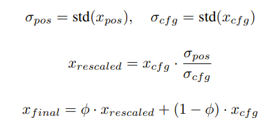
This enforces that the standard deviation of the output of the classifier-free guidance is similar to our conditioned output! So overall it won’t get overburned. Bghira did say he used a CFG of 0.7 which might also be a workaround!
Why is DeepFloyd IF pretty good here?
Now, one final fun fact. For Imagen and the Deepfloyd IF reproduction, the flaws is way less apparent. The reason for this is instead of having a linear schedule of βₜ, they instead have a cosine schedule like so
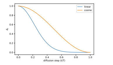
and what this causes is alpha bar at timestep T, is way closer to 1 than the linear scheduler! The table of alpha bars is as follows
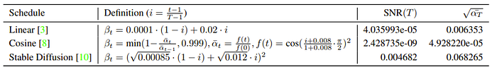
So if you don’t want to implement this issue but avoid some noisyness using a cosine schedule may be good enough. Interestingly, Imagen also had the exact same issue with classifier-free guidance which they solved by something called dynamic thresholding which was very interesting. Essentially, they push all the outputs of the model to always be in a certain range but I think the rescaling above is cleaner.
Final words
Overall, that’s it for now! I did cover the main points of the paper I was interested in but do check out the original paper here since there are parts I didn’t cover like the entire evaluation section!